The EMEP grid

According to the definition given in the Protocol on Long-term Financing of the Cooperative Programme for Monitoring and Evaluation of the Long-range Transmission of Air Pollutants in Europe (EMEP): "The geographical scope of EMEP means the area within which, coordinated by the international centres of EMEP, monitoring is carried out." This definition has been referred to in all following protocols to the Convention. Since its adoption in 1984, as Parties have ratified or acceded to the EMEP Protocol, the geographical scope of EMEP has broadened and the EMEP grid has been modified significantly two times.

From 1984 until 1997 a 150x150 km² grid were used. In 1997, the grid resolution was changed to 50x50 km², while the area covered by the finer resolution EMEP grid remained unchanged. In 2008, the 50x50 km² EMEP domain was extended. From year 2017 the spatial resolution was increased to 0.1^ox0.1^o longitude-latitude grid. The technical description of the former and present EMEP grids can be found below.

The EMEP 0.1^ox0.1^o longitude-latitude grid (2017-)

At the 36th session of the EMEP Steering Body the EMEP Centres suggested to increase spatial resolution and change the projection to a 0.1^ox0.1^o longitude-latitude EMEP grid in a geographic coordinate system (WGS84). The new EMEP domain will cover the geographic area between 30^oN-82^oN latitude and 30^oW-90^oE longitude. This domain represents a balance between political needs, scientific needs and technical feasibility. Parties are obliged to report gridded emissions in the new grid resolution from year 2017.

EMEP 0.1º x 0.1º gridded emissions and longitude-latitude definition of grid cells and fraction of grid cells per country

The extended EMEP 50x50 km² grid (2008-2016)

In 2007, the Steering Body to EMEP at its 31st session agreed to a new extension of the EMEP grid in order to include EECCA countries signatories to the LRTAP Convention. The extended EMEP 50x50 km² domain includes 132x159 points (with x varying from 1 to 132 and y varying from 1 to 159).

Download the grid description as a pdf document here.

Technical description of the EMEP 50x50 km² grid (2003-2007)

The EMEP grid system is based on a polar-stereographic projection with real area at latitude 60$^{\circ}$ N. The y-axis is oriented parallel to 32$^{\circ}$ W defined as a negative longitude if west of Greenwich. The extended EMEP 50x50 km² domain includes 132x159 points (with x varying from 1 to 132 and y varying from 1 to 159). Until 2008 the official EMEP 50x50 km² grid included only 132x111 points.

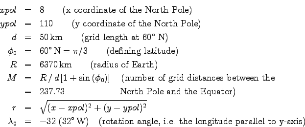
For both the extended and the former 50x50 km² grids, the latitude, φ, and longitude, λ, of any point (x, y) on the grid may be calculated as follows:

$$\begin{eqnarray*} \phi &= & 90 - \frac{360}{\pi} \arctan{\left[\frac{r}{M}\right... ...\frac{180}{\pi} \arctan{\left[\frac{x-xpol}{ypol-y}\right]} \, , \end{eqnarray*}$$

in which

$$\begin{eqnarray*} xpol & = & 8 \qquad\mbox{(x coordinate of the North Pole)} \\ ... ...d\mbox{(rotation angle, i.e. the longitude parallel to y-axis)} \end{eqnarray*}$$

The x and y coordinate in the EMEP grid of any given latitude, φ, and longitude, λ, can be found from:

$$\begin{eqnarray*} x &=& xpol + M \tan \left[\frac{\pi}{4} - \frac{\phi}{2}\right... ...frac{\pi}{4} - \frac{\phi}{2}\right] \cos{(\lambda - \lambda_0)} \end{eqnarray*}$$

It should be pointed out that x and y coordinates calculated with the equations above coincide with the grid-square centre. Thus, if a grid-square has its centre coordinates (x, y), the coordinates of its lower left and right corners are (x-0.5, y-0.5) and (x+0.5, y-0.5) respectively, and the coordinates (x, y) of its upper left and right corners are (x-0.5, y+0.5) and (x+0.5, y+0.5), respectively.

Download the grid description as a pdf document here

Technical description of the former EMEP 150x150 km² grid (-2003)

Similarly to the 50x50 km² grid, the EMEP 150x150 km² grid system is based on a polar-stereographic projection with real area at latitude 60$^{\circ}$ N. The y-axis is oriented parallel to 32$^{\circ}$ W. The EMEP 150x150 km² domain includes 44x37 points (with x varying from 1 to 44 and y varying from 1 to 37).

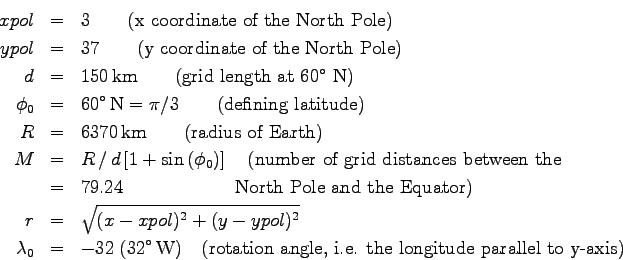
For the 150x150 km² grid, the latitude, φ, and longitude, λ, of any point (x, y) on the grid may be calculated as follows:

$$\begin{eqnarray*} \phi &= & 90 - \frac{360}{\pi} \arctan{\left[\frac{r}{M}\right... ...\frac{180}{\pi} \arctan{\left[\frac{x-xpol}{ypol-y}\right]} \, , \end{eqnarray*}$$

in which

$$\begin{eqnarray*} xpol & = & 3 \qquad\mbox{(x coordinate of the North Pole)} \\ ... ...d\mbox{(rotation angle, i.e. the longitude parallel to y-axis)} \end{eqnarray*}$$

The x and y coordinate in the EMEP grid of any given latitude, φ, and longitude, λ, can be found from:

$$\begin{eqnarray*} x &=& xpol + M \tan \left[\frac{\pi}{4} - \frac{\phi}{2}\right... ...frac{\pi}{4} - \frac{\phi}{2}\right] \cos{(\lambda - \lambda_0)} \end{eqnarray*}$$

Again, the x and y coordinates calculated with the equations above coincide with the grid-square centre. Thus, if a grid-square has its centre coordinates (x, y), the coordinates of its lower left and right corners are (x-0.5, y-0.5) and (x+0.5, y-0.5) respectively, and the coordinates (x, y) of its upper left and right corners are (x-0.5, y+0.5) and (x+0.5, y+0.5), respectively.

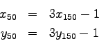
The coordinate transformation between the 150x150 km² grid and the 50x50 km² grid can be given as:

$$\begin{eqnarray*} x_{50}& =& 3x_{150}-1\\ y_{50}& =& 3y_{150}-1 \end{eqnarray*}$$

Download the grid description as a pdf document here.